PLAYING MUSICAL NOTES USING IMAGE PROCESSING
So I'm rather tired of beating around the bush every blog post so I'm just going to go straight into it! The task today is to be able to use image processing to play notes from a music score. So i scoured the web for something to use and I've chosen the following score sheet taken from [1]. Let's see if you can guess what song it is!
 |
| Figure 1. Score sheet |
 |
| Figure 2. Cropped first row |
 |
| Figure 3. Thresholded image |
Now we must have some way of identifying the type of note present. We must perform some form of blob analysis to do so. First, we close the image to close up the gaps in the half notes and then open the image to eliminate the measure lines. Note that if we did it in reverse, then the half notes would be eliminated! The code used to do this is shown in Figure 4.
1 2 3 4 5 | se1=CreateStructureElement('circle',3) se2=CreateStructureElement('circle',2) notes_play=CloseImage(notes_play,se1) notes_play=OpenImage(notes_play,se2) imshow(notes_play) |
Figure 4. Code used to eliminate the measure lines
Thus, the resulting image is shown in Figure 5. |
| Figure 5. Result after the code in Figure 4 is implemented. |
1 2 3 4 5 6 7 8 9 10 | ObjectIm=SearchBlobs(notes_play); x_cent=zeros(1,max(ObjectIm)) y_cent=zeros(1,max(ObjectIm)) for i=1:max(ObjectIm) [y,x]=find(ObjectIm==i) xmean=mean(x) ymean=mean(y) x_cent(i)=xmean y_cent(i)=ymean end |
Figure 6. Code used to find the centroid of each blob
Now that we have the centroids, we can use these centroids to find the specific pitch and timing each blob refers to! For the specific pitch, we must find the y values over within which the y component of the centroid can be present in order to be associated with a given pitch. From paint, we identify the following notes and their positions along the staff: C4 - 45, G4 - 32, A4-29, F4-35, E4-38, D4-41. Thus, allowing for this range (with a +- 2 allowance to account for errors in the centroid calculation), we can associate specific pitches to specific blogs. This was done in the code in Figure 7. The timing, on the other hand, was calculated by considering the difference between adjacent elements within the x components of the centroids. This was performed using the diff() function. If the difference between a pair of adjacent x components was greater than a certain threshold, the first occurring x centroid value was associated with a half note (and thus, a timing value of 2). Else, the note is given a timing value of 1 for a quarter note. Note that because there is no element AFTER the last element (the very definition of being "last"), the timing of the last note had to be hard coded.
1 2 3 4 5 6 7 8 9 10 11 12 13 14 15 16 17 18 19 20 21 22 23 24 25 26 27 28 29 30 31 32 33 | note=zeros(1,size(y_cent,2)) for j=1:size(y_cent,2) if y_cent(1,j)>44 & y_cent(1,j)<46 note(1,j)=261.63 end if y_cent(1,j)>31 & y_cent(1,j)<33 note(1,j)=196*2 end if y_cent(1,j)>28 & y_cent(1,j)<31 note(1,j)=220*2 end if y_cent(1,j)>34 & y_cent(1,j)<36 note(1,j)=349.23 end if y_cent(1,j)>37 & y_cent(1,j)<39 note(1,j)=329.63 end if y_cent(1,j)>40 & y_cent(1,j)<42 note(1,j)=293.66 end end spacing=diff(x_cent) timing=zeros(1,size(x_cent,2)) for j=1:size(spacing,2) if spacing(j)>60 timing(j)=2 end if spacing(j)<60 timing(j)=1 end end timing(1,14)=2 |
Figure 7. Code used to generate the timing and note information for playback
Now, using the timing and note arrays, we can finally play the music! We utilize the function given to us by Ma'am Jing.
1 2 3 4 5 6 7 8 9 | function n = note_func(f, t) n = sin(2*%pi*f*linspace(0,t,8192*t)); endfunction; v=[] for i=1:size(note,2) v=cat(2,v,note_func(note(1,i),(timing(1,i)))) end sound(v,8192) |
Figure 8. Code used to generate the sounds
Playing the above file with all the other code will yield to the correct output! In case you don't have Scilab at the moment, try listening to it here. Note that we used a sampling frequency of 8192 samples/second and thus, each quarter note is given 1 second while each half note is given 2 seconds.
How does it sound? The pitches and timing sound on point, but there just seems to be some digital feel to it. This is due to the fact that we are playing sinusoids of constant frequency AND amplitude. Sounds produced by real world instruments are still mostly composed of single frequency sinusoids, but their amplitudes are modulated by envelope functions. These exact form of these envelope functions are specific to the instruments used but are generally piecewise functions composed of four segments: an attack, a sustain, a decay, and a release. A sample envelope function is shown in Figure 9.
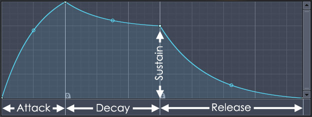 |
| Figure 9. Sample envelope function taken from [2]. |
We can attempt to apply an envelope function to our sinusoids in order to make them sound more realistic. To do this, we refer to [3] for typical time values of each segment of the envelope function. For a total time of one second, employ an attack time of 0.05 seconds, a slight sustain of 0.10 seconds, a slight 10% decrease over 0.10 seconds, a 50% decay over 0.70 seconds, and a turning off time of 0.05 seconds. Because we have 8192 samples per second, this corresponds to approximately 410 samples each for the attack and turning off, 819 samples each for the slight sustain and decrease, and 5734 samples for the decay. We approximate each segment by a straight line. The graph of this envelope function is shown in Figure 10 and the resulting modified note_func() function is shown in Figure 11.
 |
| Figure 10. Envelope function to be used |
1 2 3 4 5 6 7 8 9 10 | function n = note_func(f, t) n = sin(2*%pi*f*linspace(0,t,8192*t)); line1 = linspace(0, 1, 410*t); line2 = linspace(1, 1, 819*t); line3 = linspace(1, 0.9, 819*t); line4 = linspace(0.9, 0.45, 5734*t); line5 = linspace(0.45, 0, 410*t); envp=[line1,line2,line3,line4,line5]; n=n.*envp endfunction; |
Figure 11. Modified note_func() function to include the envelope function
Now let's take a listen to the output here. Sounds way more realistic right? Now that I didn't encounter any rest stops in the sheet music I tested, but I guess we could "play" a rest stop by setting its frequency to a value outside of the human audible range (20Hz to 20kHz).
I have to admit: I was pretty frustrated with this activity. This wasn't because the activity was hard or anything, but it was cause my Scilab failed me once again. Adding to a lot of things I've gained this semester, I've grown to hate Scilab hahahaha. I really wish I had more time to do this blog as I found the activity pretty cool. Maybe I'll work on a similar project over the Christmas break! Anyway, despite this, I was still able to finish the activity. The output was pretty good and I believe I applied the past image processing techniques well. I pretty much understood what I was doing and presented the steps in a logical manner. Also, taking the extra step to apply an envelope function to make the notes sound more "real" is a plus. For this, I'd give myself a 12/10.
Acknowledgements:
I'd like to acknowledge Mich Medrano's blog for helping me setup my note playing function such that the t argument could be set in seconds. I'd also like to thank Roland Romero for providing me with the reference to help in generating an envelope function.
References:
[1] (n.d.). Retrieved December 7, 2016, from http://clarinetsheetmusic.net/title/t/twinkle-twinkle-little-star/twinkle-twinkle-little-star.gif
[2] Envelope. (n.d.). Retrieved December 07, 2016, from https://www.image-line.com/support/FLHelp/html/glossary_envelope.htm
[3] How to Create a Wave File using Scilab. (n.d.). Retrieved December 07, 2016, from http://www.lumanmagnum.net/physics/sci_wav.html
No comments:
Post a Comment